
Inbreeding Coefficient
Published:
The inbreeding coefficient is a measure of the probability that an individual’s two alleles are identical by descent (IBD) because the parents share common ancestors. It is usually denoted by \(F\). If the two parents are unrelated, \(F = 0\). If the parents are related (e.g. half-sibs, full sibs, cousins), the offspring is more likely to inherit the same allele from a common ancestor, so \(F > 0\). The larger \(F\) is, the higher the degree of inbreeding.
Methods of calculation
Path method (Wright’s method)
Theory
The path method is the classical approach. It is very intuitive when the pedigree is small or when used for teaching. The formula is:
\[F_X = \sum \left(\frac{1}{2}\right)^{n_1+n_2+1}(1+F_A)\]- \(n_1\): number of generations from father to the common ancestor
- \(n_2\): number of generations from mother to the common ancestor
- \(F_A\): inbreeding coefficient of the common ancestor
Example
We use an example generated with the quickped project:
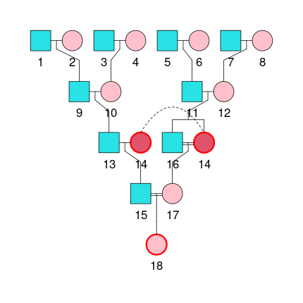
Blue squares and red circles denote males and females respectively. We compute the inbreeding coefficient of individual 18. The path method requires finding all distinct paths and summing their contributions.
Step 1. Identify the parents of individual 18: 15 and 17.
Step 2. Find the common ancestors of 15 and 17: 14, 11, and 12.
Step 3. Find all distinct paths and compute each:
Path A — through common mother 14
- Path: \(15 \leftarrow \mathbf{14} \rightarrow 17\)
- Generations: 15 → 14: 1; 17 → 14: 1
- Contribution: \(\left(\frac{1}{2}\right)^{1+1+1}(1 + F_{14}) = \left(\frac{1}{2}\right)^3(1 + 0) = 0.125\)
- Note: Individual 14 is the common mother of 15 and 17 and gives the shortest inbreeding path.
Path B — through common grandfather 11
- Path: \(15 \leftarrow 13 \leftarrow \mathbf{11} \rightarrow 16 \rightarrow 17\)
- Generations: 15 via 13 to 11: \(n_1 = 2\); 17 via 16 to 11: \(n_2 = 2\)
- Contribution: \(\left(\frac{1}{2}\right)^{2+2+1}(1 + F_{11}) = \left(\frac{1}{2}\right)^5(1 + 0) = 0.03125\)
Path C — through common grandmother 12
- Path: \(15 \leftarrow 13 \leftarrow \mathbf{12} \rightarrow 16 \rightarrow 17\)
- Generations: 15 via 13 to 12: \(n_1 = 2\); 17 via 16 to 12: \(n_2 = 2\)
- Contribution: \(\left(\frac{1}{2}\right)^{2+2+1}(1 + F_{12}) = \left(\frac{1}{2}\right)^5(1 + 0) = 0.03125\)
Step 4. Sum contributions from all paths:
\[F_{18} = \text{Path A} + \text{Path B} + \text{Path C} = 0.125 + 0.03125 + 0.03125 = 0.1875\]Diagonal matrix method & recursion (Meuwissen & Luo, 1992)
Theory
\[F_i = A_{ii}-1\]\(A_{ii}\) is the diagonal element of the numerator relationship matrix.
Example
Using the same pedigree (0 denotes unknown):
Pedigree:
| ID | Sire | Dam | Sex |
|---|---|---|---|
| 1 | 0 | 0 | 1 |
| 2 | 0 | 0 | 2 |
| 3 | 0 | 0 | 1 |
| 4 | 0 | 0 | 2 |
| 5 | 0 | 0 | 1 |
| 6 | 0 | 0 | 2 |
| 7 | 0 | 0 | 1 |
| 8 | 0 | 0 | 2 |
| 9 | 1 | 2 | 1 |
| 10 | 3 | 4 | 2 |
| 11 | 5 | 6 | 1 |
| 12 | 7 | 8 | 2 |
| 13 | 9 | 10 | 1 |
| 14 | 11 | 12 | 2 |
| 15 | 13 | 14 | 1 |
| 16 | 11 | 12 | 1 |
| 17 | 16 | 14 | 2 |
| 18 | 15 | 17 | 2 |
Some useful facts: the relationship between parent and offspring is 0.5, and between full sibs is 0.5. Using the parent–offspring relationship of 0.5, we can fill part of the matrix.
Reduced relationship matrix (6×6); the same rules extend to 18×18:
| 13 | 14 | 15 | 16 | 17 | 18 | |
|---|---|---|---|---|---|---|
| 13 | 1.0000 | 0.0000 | 0.5000 | 0.0000 | 0.0000 | 0.2500 |
| 14 | 0.0000 | 1.0000 | 0.5000 | 0.5000 | 0.7500 | 0.6250 |
| 15 | 0.5000 | 0.5000 | 1.0000 | 0.2500 | 0.3750 | 0.6875 |
| 16 | 0.0000 | 0.5000 | 0.2500 | 1.0000 | 0.7500 | 0.5000 |
| 17 | 0.0000 | 0.7500 | 0.3750 | 0.7500 | 1.2500 | 0.8125 |
| 18 | 0.2500 | 0.6250 | 0.6875 | 0.5000 | 0.8125 | 1.1875 |
Off-diagonal elements are computed by recursion:
\[A_{ij} = \frac{1}{2}A_{s(i),j} + \frac{1}{2}A_{d(i),j}\]where \(s(i)\) is the sire of individual \(i\) and \(d(i)\) is the dam. Diagonal elements:
\[A_{ii} = 1 + \frac{1}{2}A_{s(i),d(i)}\]Recursion (abbreviated):
- Base: \(a_{13,14}=a_{14,13}=0\), \(a_{13,13}=1\), \(a_{14,14}=1\)
- Individual 15: \(a_{14,15}=a_{15,14}=0.5\), \(a_{15,13}=a_{13,15}=0.5\), \(a_{15,15}=1\)
- Individual 16: \(a_{14,16}=a_{16,14}=0.5\), \(a_{15,16}=a_{16,15}=0.25\), \(a_{16,16}=1\)
- Individual 17: \(a_{14,17}=a_{17,14}=0.75\), \(a_{15,17}=a_{17,15}=0.375\), \(a_{16,17}=a_{17,16}=0.75\), \(a_{17,17}=1.25\)
- Individual 18: \(a_{13,18}=a_{18,13}=0.25\), \(a_{14,18}=a_{18,14}=0.625\), \(a_{15,18}=a_{18,15}=0.6875\), \(a_{16,18}=a_{18,16}=0.5\), \(a_{17,18}=a_{18,17}=0.8125\), \(a_{18,18}=1.1875\)
Then, from the diagonal method:
\[F_i = A_{18,18}-1 = 1.1875 - 1 = 0.1875\]References
- Wright, S. (1922). Coefficients of inbreeding and relationship. The American Naturalist, 56(645), 330–338.
- Henderson, C. R. (1976). A simple method for computing the inverse of a numerator relationship matrix used in prediction of breeding values. Biometrics, 32(1), 69–83.
- Meuwissen, T. H. E., & Luo, Z. (1992). Computing inbreeding coefficients in large populations. Genetics Selection Evolution, 24(4), 305–313.